
LIME: explain Machine Learning predictions
Giorgio Visani
Intuition and Geometrical Interpretation of LIME
LIME stands for Local Interpretable Model-agnostic Explanations. It is a method for explaining predictions of Machine Learning models, developed by Marco Ribeiro in 2016 [3].
As the name says, this is:
- Model Agnostic: works for any kind of Machine Learning (ML in the following) model. More on model agnostic tools here.
- Local: aims at explaining only a small part of the ML function.
In the following, we are going to review the steps of LIME algorithm, to be on the same page when we will consider the intuition behind the method.
In order to get the most out of it, be sure to have well in mind the Geometrical Perspective of ML models (☍).
LIME Algorithm
- Choose the ML model and a reference point to be explained
- Generate points all over the ℝᵖ space
(sample X values from a Normal distribution inferred from the training set) - Predict the Y coordinate of the sampled points, using the ML model
(the generated points are guaranteed to perfectly lie on the ML surface) - Assign weights based on the closeness to the chosen point
(use RBF Kernel, it assigns higher weights to points closer to the reference) - Train Linear Ridge Regression on the generated weighted dataset:
E(Y)= β₀ + ∑ βⱼ Xⱼ. The β coefficients are regarded as LIME explanation.
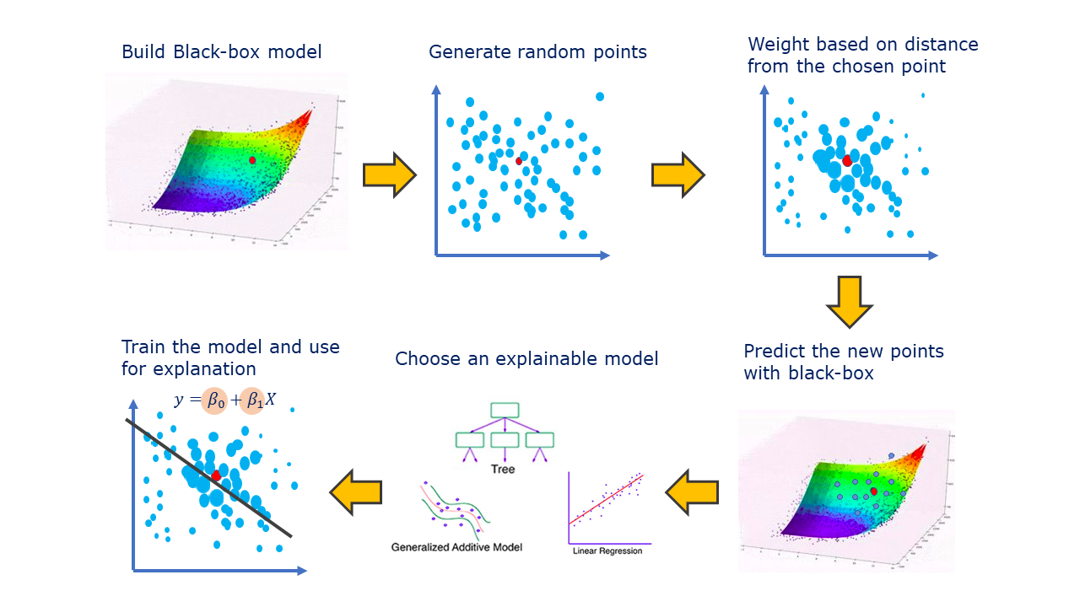
LIME explanation is valid only in the neighborhood of the reference individual (red dot).
Generation Step
LIME generates n points xᵢ′ all over the ℝᵖ space of the X variables, also in faraway regions from our red point. — xᵢ′ stands for the LIME generated points, while xᵢ are the observations of the original dataset — We generate only the X values for the n points xᵢ′, but we miss the Y value for the new units. So we plug each xᵢ′ into the ML model and we obtain its prediction for the new point: ŷᵢ′. We actually generated a brand-new dataset.
Because the Y is computed using the ML model, we are guaranteed that the new points perfectly lie on the ML surface! Basically, we have now a dataset representing our ML surface for some scattered points all over the ℝᵖ⁺¹ geometrical space.
Since we are not interested in faraway points (LIME is a local method), we must ignore them. How to do it?
LIME gives a weight to each generated point, using a Gaussian (RBF) Kernel.

The Gaussian Kernel attributes a value in the range [0,1], the higher the closer to the reference point. The kernel width kw parameter decides how large is the circle of the meaningful weights around the red dot.
White dots are the original dataset points, red dot is the reference point and the blue line is the prediction function of the ML model. Green circles show how the kernel weights are assigned, based on the kernel width parameter: the inner circle gives meaningful weights only to very close units because kw is low, the outer circle employs a larger kw. Picture by the author
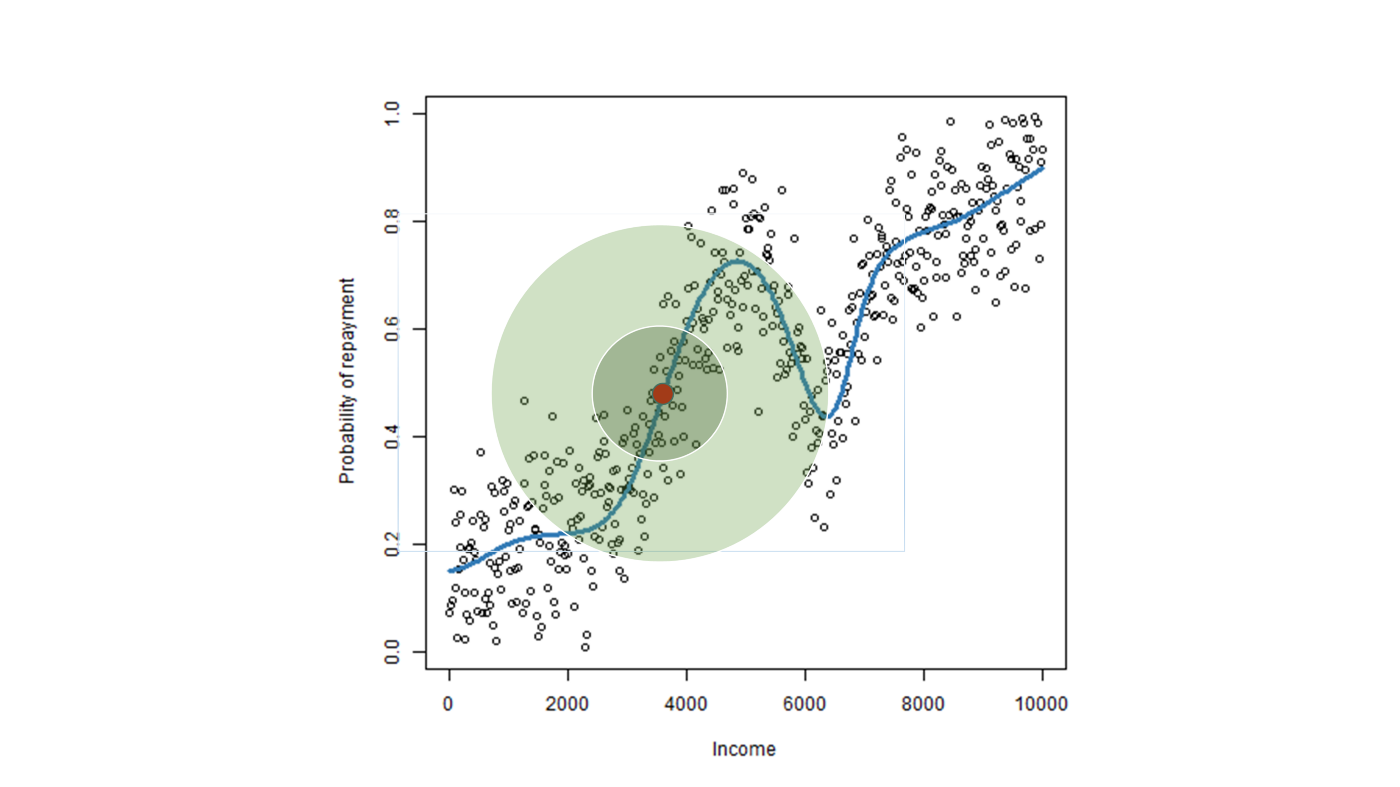
Thanks to the weights, we understand if the points are far away or close to the red dot.
Local Explainable Model Step
LIME is now ready to use a surrogate model to approximate the ML model in the small region around our reference red dot, determined by the Kernel weight. We may choose any kind of explainable model for the approximation (Decision Trees, Logistic Regression, GLM, GAM, etc), although my preference is for Linear Regression (it can be viewed as the tangent to ML [☍]).
— The default surrogate model in LIME’s Python implementation is Ridge Regression, which belongs to the Linear Regression class of models — .
The explainable model is usually exploited to understand which variables are the most important for the ML prediction for the specific individual (comparing the coefficients of the variables). But LIME models can also be used to test what-if scenarios ( eg. If I were to earn 500$ more a year, how many points would I gain on my credit score?). It is important to remember that the surrogate model is only valid locally: the scenario we test should be not too distant from our reference. Such what-if tool is available only for surrogate models: it cannot be done for other explainable methods such as the ones based on feature attribution, because they don’t rely on prediction models.
Intuition
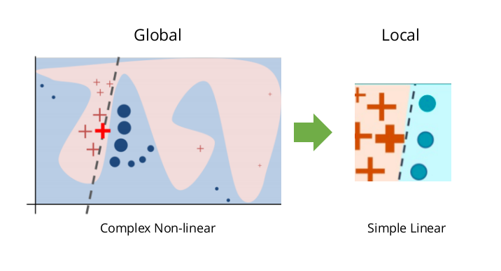
Since we have a complex and wiggly prediction curve f(x), obtained by the ML model, LIME's goal is to find its tangent at a precise point (the reference individual).
From Taylor Theorem, we know that each function f can be approximated using a polynomial. The approximation error depends on the distance from the reference point and on the degree of the polynomial (higher degree ensures lower error).
The tangent corresponds to the Taylor polynomial of degree 1, the simplest. Since it is the lowest polynomial degree, to obtain a good approximation we should consider a small region around the reference — the smaller the more accurate is the linear approximation of f(x) — .
For more intuition about first-order Taylor approximation, check out this.
So, all in all, it is just a tangent. Why LIME is not computing the tangent analytically? It would just require to calculate the derivative to the f(x) function. It would be simpler (allowing to get rid of the entire generation step) and less time-consuming.
Unfortunately, as explained here, ML does not provide the formula of the prediction function f(x). Without the formula, it is impossible to calculate the derivative!!
LIME basically reconstructs a part of the f(x) function, using the generation step, and approximates its derivative with Linear Regression.
LIME weak points
The generation step is an open issue!
The current implementation generates points all over the ℝᵖ space of the X variables, then gives importance only to the close ones, using the RBF Kernel with the proper kernel width kw value.
Two questions arise naturally:
- Why don’t just generate only points close to the reference?
- How to choose the correct value for the kernel width?
Why don’t just generate points close to the reference?
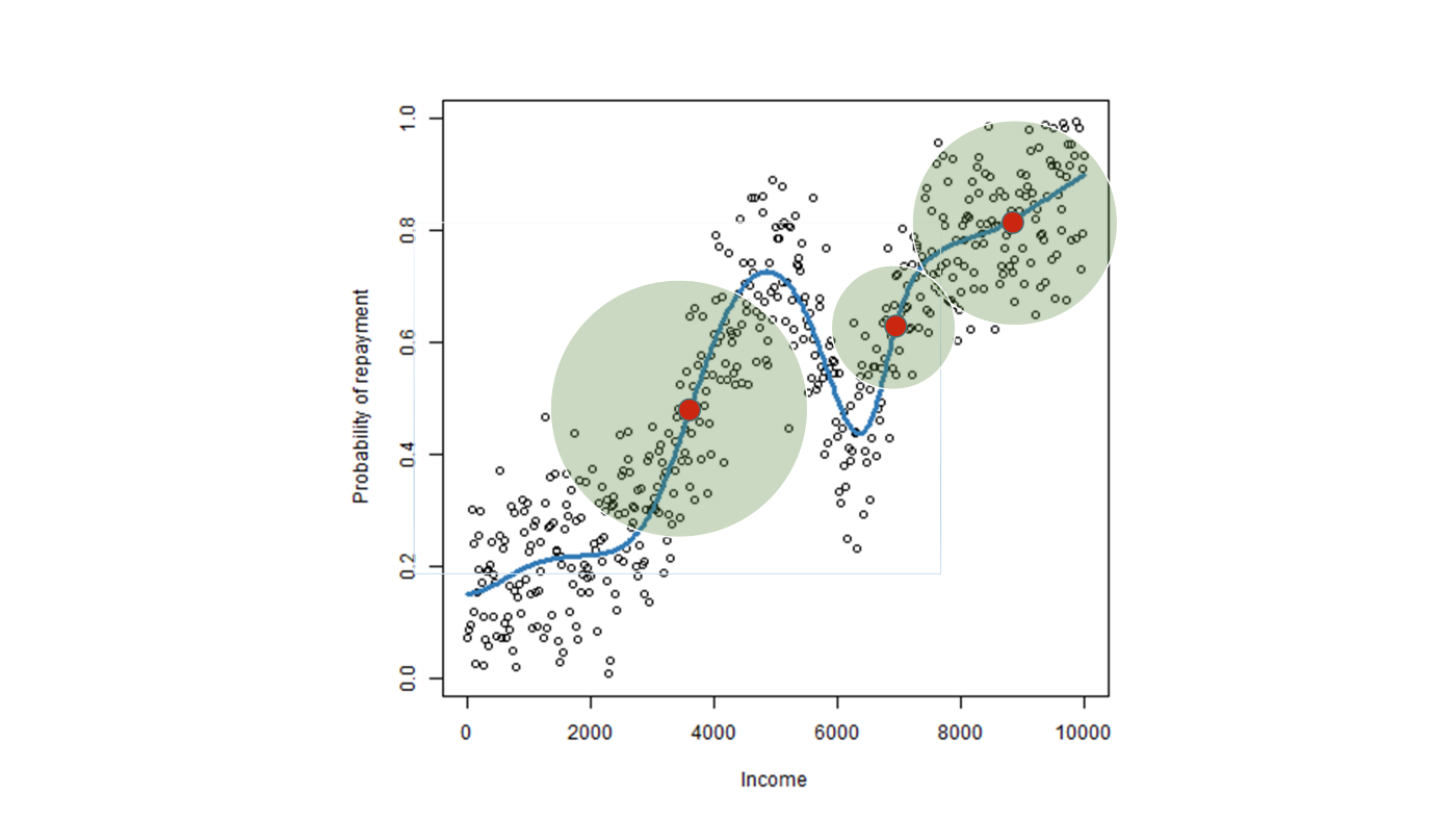
This is a delicate subject: in principle, it would be better to consider only the points in the region of interest, although the proper size of the region is not fixed but depends on the reference point.
In fact, the neighborhood should include all the linear area of the ML curve around the reference point, therefore it depends on the local curvature of f(x).
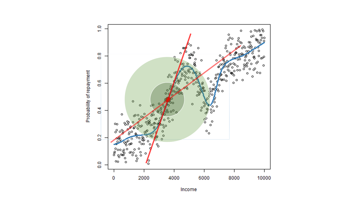
In the Picture below you may see how different points have different proper size for the linear local region.
There are some works on local generation techniques for LIME (in particular Laugel and Renard’s work [2] and Guidotti’s LORE [3] technique). Unfortunately, both of them still present issues. The first paper considers other factors in the method development, losing the important concept of the tangent. The second one, instead, does not guarantee to consider the entire linear area around the reference dot (it just finds a very small neighborhood, without checking if the ML function is linear also a little bit further). This is a big drawback because small neighborhoods cause LIME explanations to be unstable.
How to choose the correct value for the kernel width?
This is considered the biggest issue, for some time the practitioners just tried out many different values and checked whether the explanations were reasonable.
This is clearly a problem: we are not sure the trained ML model makes reasonable decisions. So, if the ML finds strange or unreasonable rules, we expect LIME to be unreasonable too (after all that is precisely why we use LIME: to understand ML behavior and potential ML issues).
But if we choose the kw value based on meaningful explanations, we won’t be able to spot any ML problem!!
Moreover, we can see how bad choices of the kernel width distort the LIME line, making it very different from the tangent (as in the Picture below).
[1] Guidotti, R., Monreale, A., et al. , 2018. Local rule-based explanations of black box decision systems, ArXiv preprint
[2] Laugel, T., Renard, X., Lesot, M.-J., Marsala, C., Detyniecki, M., 2018. Defining locality for surrogates in post-hoc interpretablity. WHI Workshop @ ICML
[3] Ribeiro, M.T., Singh, S., Guestrin, C., 2016. “ Why should I trust you?” Explaining the predictions of any classifier. SIGKDD
[4] Visani, G., Bagli, E., Chesani, F., 2020. OptiLIME: Optimized LIME Explanations for Diagnostic Computer Algorithms. AIMLAI Workshop @ CIKM


