Explainable Machine Learning
Giorgio Visani
XAI Review: Model Agnostic Tools
In the last few years, there has been a lot of fuss about how to explain Machine Learning (ML) predictions. Methods and techniques have been developed at an incredible pace in the last 5 years, so much that now there is an entire field about it: XAI (eXplainable Artificial Intelligence).
The basic goal of XAI is to describe in detail how ML models produce their prediction, since it is of much help for different reasons. The most important are
- Data Scientists who build the model may benefit from understanding how it behaves, so they may modify parameters accordingly, to improve the model’s accuracy and fix prediction bugs,
- In many fields, there exists a regulator which should validate the model before it is possible to use it in production. Nowadays, a bunch of regulations require to provide explanations for the model, such as GDPR and the Ethics Guidelines for Trustworthy AI,
- People affected by the model may ask for the drivers of their prediction.
A good explanation may generate more trust into Machine Learning, which is considered by someone as a “big bad guy”.
These very good motivations explain why XAI is such a hot topic nowadays. Let’s now dive deep into the techniques and options we have at hand.
Approaches to Interpretability
There are basically two approaches to achieve Interpretability:
- you may actually build a Transparent ML model (one which is understandable without further intervention)
- or you could use a black-box model ad apply a Post-Hoc technique on top of it, to explain its very complex behavior
Transparent Models
Nowadays the Transparent ML world is a hot research topic (if interested I suggest to read some of Cynthia Rudin’s works like [6], as well as[1] from Alvarez-Melis), however, they don’t look like being ready to replace complex black-box models, which have been studied for the last 20 years and are proven to be very good for many tasks.
Moreover, I bet it is more trendy to use a very complex Gradient Boosting or Neural Network model, instead of classical Logistic Regression or Decision Trees (it is also a way to impress your client with new powerful stuff).
Post-Hoc Techniques
Said so, here we are going to focus on Post-Hoc Techniques, i.e. explanation methods that work on top of complex black-box methods. So that anyone can have fun with the ML model he prefers.
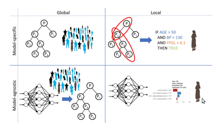
Post-Hoc Methods are partitioned following two main concepts: Model Agnostic/Model Specific and Local/Global techniques.

I’m a big fan of Model Agnostic Techniques: no matter what ML model you used before, they will provide you an explanation for it. Now, have you ever wondered how it is possible? Here’s the answer:
Geometrical Interpretation of Prediction model
Basically, each prediction model (be it Machine Learning, Statistical, etc.) draws a prediction function f(x): given a set of x values, it returns the forecasted ŷ.
In the following, I will convince you of this and give some insight regarding the different shapes of prediction functions obtained from different models.
The main reason for using ML is to get insight on how the Y variable changes its values depending on the values of the X variables. So we are assuming Y depends on the Xs (what we’re saying is the Xs are the cause of Y and not the other way around! The direction of the causal relation is not checked in the standard ML models).
All in all, we are interested in the function encoding the dependence between Y and X.
et’s now consider the variables used in the prediction models.
The first thing that catches the eye is we can turn into numbers almost any kind of info:
- images represented as pixels intensity colors ranging from 0 to 255,
- words and text embedded into latent semantic spaces of concepts,
- categories encoded as dummies, etc.
Hence, we only deal with numeric features when the bare ML algorithm is employed! The features in the dataset can be viewed as one dimension of a geometric space, where p is the number of X features in the dataset and the additional dimension is the Y variable.
The observations of our dataset are points in such ℝᵖ⁺¹ space. Therefore, the prediction function f(x) is the surface that best approximates all the points in the geometric space, while at the same time, it represents the best guess about the causal relationship existing between Y and the Xs.
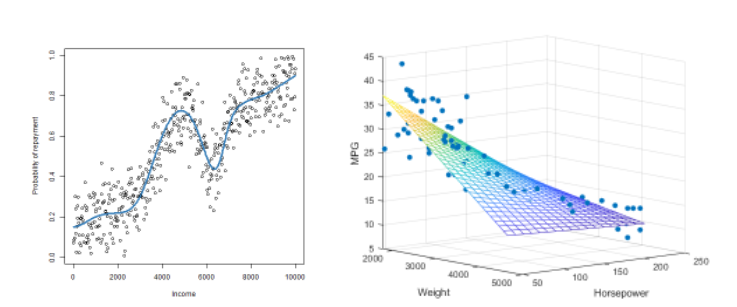
Just to give you a hint of this, I’ll show you some prediction functions f(x) obtained using different ML models:
Each prediction technique produces the f(x), the difference between ML algorithms is in the f shape.

Standard statistical methods usually put constraints on the shape (eg. Linear Regression requires to create a linear plane, as in Figure above, Logistic Regression allows f to be non-linear, but strictly increasing or decreasing (monotonic) so it may not achieve a curly f as in the left picture, etc.).
These methods are called parametric because we choose the formula for f and we just look for the best coefficients: as an example, Linear Regression’s f has formula Y =β₀ +β₁ X₁ + β₂ X₂, we can select the best values for β₀, β₁, β₂. But we won’t ever achieve a formulation in which the X₁ has a wavy behavior.
Strictly speaking, they are less powerful because they are constrained in some way. But their advantage is in their simplicity: they create simple surfaces which can be expressed with an easy function.
Even more important, they provide you with the formula for f. With it, we can understand very well how the function behaves also without looking at the picture of the geometrical space!
Instead, complex ML models, such as Gradient Boosting, Neural Networks, Random Forests, are non-parametric methods: they give f the freedom to fully modify its shape, which can become wiggly at will, as well as understand well the correlation and interaction between X variables.
Thanks to this peculiarity, they usually achieve better or at least equal prediction, compared to Statistical models. Unfortunately, the biggest strength turns also into the worst weak point: we do not get back the precise f formula! When we have just 1 or 2 X variables we may draw f on the geometrical space, but when it is more we have no way to understand the surface.
Core message: any ML technique builds the best function f(x) to approximate our data, given the constraints. Some of them produce simple f(x) and they also return the formula, while the black-box ones create very complicated functions and do not provide the math formula.
Model Agnostic Explanations
These techniques try to give some insight about the f(x) function underlying the model, regardless of the model structure.
This can be done for each ML algorithm, since all of them exploit the prediction function concept.
Each model agnostic method makes use of a brilliant idea to give some intuition/understanding/other info about f(x).
Let’s consider some of the core ideas underlying various techniques:
- SURROGATE MODELS constitute a very big class of explanation techniques. The basic concept is to approximate the function f(x) with another model, this time the new model should be explainable.
Some methods are global — try to approximate f(x) on all the ℝᵖ⁺¹ space — while the local ones require you to choose a small region of the space and give an approximation of just that part of the curve. Clearly, there is a lot of freedom on which interpretable model to choose and how to assess whether the approximation to the ML function is good.
An example of the Global ones is Trepan [5], which approximates f(x) using a Decision Tree.
For the Local methods, a very famous one is LIME (Local Interpretable Model agnostic Explanations). - Another big class is based on the FEATURE IMPORTANCE: the idea is to give an importance value to each variable, depending on how much it influences the f(x). The important point here is how to find a rightful way to decompose the importance between variables (variables may be correlated as well as interact with each other).
One of the big ideas is to consider one variable at a time and exclude it from the model. We expect to lose prediction power if the variable was important, while a negligible variable won’t make big changes. Further refinements to this idea have been proposed over the year to take into account correlated variables and interactions.
PDP [3], ALE [2], ICE [4] plots are global methods exploiting this idea, while Shapley Values [8](and its famous approximation to make them computable, SHAP [7]) rely on it for local explanations.
To recap
In this article, we reviewed the main ideas underlying Model Agnostic explanations for Machine Learning models. In particular, we focused on the geometric interpretation of the models, which I consider the building brick of many different techniques. In the next articles, we will use these basic notions to explore deeply specific frameworks: in particular, we will talk about LIME (since I’ve been working on this method for the past year).
[1] Alvarez Melis, D., Jaakkola, T., 2018. Towards robust interpretability with self-explaining neural networks, NIPS
[2] Apley, D.W., Zhu, J., 2020. Visualizing the effects of predictor variables in black box supervised learning models, Journal of the Royal Statistical Society
[3] Friedman, J.H., 2001. Greedy function approximation: a gradient boosting machine, Annals of statistics
[4] Goldstein, A., Kapelner, A., Bleich, J., Pitkin, E., 2015. Peeking inside the black box: Visualizing statistical learning with plots of individual conditional expectation, JCGS
[5] Craven, M., Shavlik, J., 1995. Extracting tree-structured representations of trained networks. NIPS
[6] Lin, J., Zhong, C., Hu, D., Rudin, C., Seltzer, M., 2020. Generalized and Scalable Optimal Sparse Decision Trees, ICML
[7] Lundberg, S.M., Lee, S.-I., 2017. A unified approach to interpreting model predictions, NIPS
[8] Shapley, L.S., 1953. A value for n-person games. Contributions to the Theory of Games


